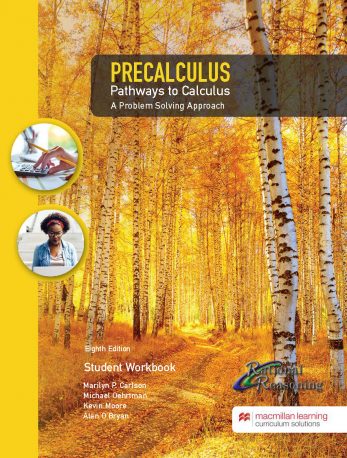
The Pathways Precalculus curriculum consists of 12 modules. Each module contains 6 to 12 in-class investigations that include problems and prompts that engage students in making meaning, building connections and understanding ideas. Students learn general approaches for solving problems that enable them to emerge as competent and confident problem solvers.
The optional Module 1 includes skill practice and a review of basic formulas. The second module helps all students solidify their understanding of ideas of quantity, variable, rate of change, and formula that are necessary for succeeding in and learning precalculus and calculus. Students learn to use their own reasoning to develop meaningful formulas and graphs to represent the patterns (linear, quadratic, exponential, trigonometric) of how two quantities change together. As students move through the course they are supported in understanding inverse functions (e.g., logarithmic function, arsine) as a reversal of the function process after learning the meaning of and methods for solving equations. Students develop confidence and competence in their ability to develop and interpret function formulas and graphs to represent quantitative relationships in applied contexts.
The online textbook includes conceptual explanations and questions, many engaging examples, and short videos that explain how to approach and solve novel problems. Linked interactive animations and applets are included to support students in approaching applied problems by conceptualizing relevant quantities and how they are related, prior to defining variables or constructing a formula or graph.
Module 1. Practicing Symbolic: Reasoning
Evaluating, Simplifying and Solving: A Conceptual and Practice Oriented Review. We review methods and rationale for evaluating and simplifying expressions and solving equations. Practice problems and detailed solutions provide all students opportunity to gain fluency with procedural aspects of algebra. Basic geometric formulas are also reviewed and students practice combining formulas for the purpose of relating two quantities that cannot be directly related with a standard formula.
Module 2. Reasoning About and Representing Quantitative Relationships
Quantity, Variable, Proportion and Linearity: Students learn to identify and relate quantities in applied contexts. The idea of variable is introduced as a way of representing the value of a varying quantity (e.g., Jane’s number of feet from the mailbox, the number of seconds since the starting gun was fired in the race) can assume. Students are introduced to the ideas of constant rate of change and average rate of change, and learn to use these ideas to construct meaningful formulas, tables and graphs that relate two covarying quantities. The meaning of and techniques for solving equations are discussed and applied. Students explore the distance formula and use the Pythagorean theorem to compute distances that cannot be directly measured.
Module 3. Formalizing Relationships Between Quantities: Functions
Students are introduced to the idea of function as a more formal way of describing and representing how the values of the function’s input quantity are related to the values of the function’s output quantity. The idea of function composition is introduced as a chaining together of two function processes for the purpose of relating two specified quantities. We introduce the idea of function inverse as an undoing of the function process. We present methods for composing and inverting functions that are represented as formulas, graphs and tables, with emphasis on using function composition and function inverse purposefully to solve novel problems.
Module 4. Exponential and Logarithmic Functions
A Multiplicative Approach: Students are introduced to exponential functions by contrasting multiplicative growth (growth that builds on itself) with growth that accumulates by adding constant amounts. The multiplicative growth of an exponential function is explored in the context of population growth, compound interest, radioactive decay and other applications. Students learn to construct meaningful exponential functions by understanding how to represent the base (growth factor) and initial value of an exponential function in both algebraic and graphical forms. The idea of the “nth root” of a number is reviewed as a means of determining the base of an exponential function for arbitrary intervals of the independent quantity (e.g., the 1 month decay factor when the 1 year decay factor is known). We introduce the ideas of logarithm and logarithmic function as the inverse of an exponential function, and as a means of representing the number of factors of a designated base needed to represent a number. We also address notational issues of representing both exponential and logarithmic functions from the perspective of the meaning conveyed by the symbols.
Module 5. Polynomial and Power Functions
Connections Across Function Representations. Students are introduced to the general form of polynomial functions and learn to reason about how a polynomial function grows as the input quantity grows without bound in both the negative and positive directions. The proportional growth patterns of linear polynomial functions are contrasted with those of non-linear polynomial functions. Students explore the average rate of change of polynomial function over fixed contiguous intervals of a function’s domain. These explorations lay the groundwork for understanding ideas of concavity, changing rate of change, and inflection points on a graph. Students explore the growth pattern and special properties of quadratic functions; they also learn methods for determine the maximum and minimum of a quadratic function. Students are also introduced to methods for graphing polynomial functions, including approaches for finding a function’s roots, maximums, and minimums. Students practice factoring and solving in contexts that are meaningful for determining zeros and roots.
Module 6. Rational Functions and an Introduction to Limit
Students explore growth patterns of rational functions by continuing to reason about how the values of two quantities change together. We examine the long-run behavior of rational functions by investigating what the function gets close to, as the input quantity grows without bound in both the negative and positive directions. Examining a function’s behavior as it gets closer and closer to some value(s) of the input variable that makes the function undefined provides a conceptual approach to understanding the behavior of rational functions near these function values. Methods for determining asymptotes emerge out of these explorations.
Module 7. Angle Measure and Trigonometric Functions
Students are introduced to the ideas of angle and discover methods for determining an angle’s measure by investigating approaches for measuring the openness of an angle’s two rays. We introduce methods for modeling the behavior of periodic motion in the context of co-varying an angle measure with a linear measurement that maps out a periodic motion, laying the groundwork for introducing the trigonometric functions of sine, cosine and tangent. Students develop an understanding of trigonometric functions in a unit circle context, and then use these functions to model periodic motion in applied contexts. The module concludes by exploring the meaning of period, amplitude, and translations of both the sine and cosine functions.
Module 8. Right Triangle Trigonometry
Students are introduced to right triangle by exploring the right triangle relationships defined by sine, cosine, and tangent functions in a unit circle context. Students are supported in seeing the connections between unit circle and triangle trigonometry. TI1e triangle relationships defined by the sine, cosine, and tangent functions are used to define relationship and determine the values of unknown quantities in applied contexts. We conclude the module by deriving various trigonometric identities that relate the trigonometric functions to one another. We also develop and use the Law of Sines and Law of Cosines to determine unknown quantities in non-right triangle contexts.
Module 9. Polar Coordinates
Students are introduced to polar coordinates by initially exploring contexts that illustrate the usefulness of polar coordinates as an alternate coordinate system. They then practice graphing and interpreting polar functions by tracking the co-variation of distances and directions. Students examine the idea of constant rate of change in the polar coordinate system. They then explore the meaning of average rate of change for functions defined in polar coordinates. After working with average rates of change, students are introduced to methods for converting between rectangular and polar coordinates, and converting functions defined in one coordinate system to a function in the other coordinate system.
Module 10. Vectors
The idea of vector is introduced in applied contexts with quantities that have both a direction and magnitude. Students investigate vector addition as a way of determining the net effect of multiple vectors interacting with one another. Students represent a vectors in both polar form and component (or rectangular) form. Students also learn how to scale vectors (the process of changing the magnitude of a vector by some factor) with both positive and negative scalars.
Module 11. Sequences and Series
Students review the idea of sequence as a function relationship between term values and term positions. They graph sequences by generating ordered pairs consisting of the position and value of the terms and are introduced to notation for describing sequences using both recursive and explicit formulas. We apply these ideas by developing the meaning of arithmetic and geometric sequences and develop formulas to represent them. We then define what we mean by a series and use sequences of partial sums to keep a running total of the sum of the terms of the sequence. The module concludes by establishing sigma notation as a way of representing a series and by developing methods for finding the sums of finite arithmetic series, finite geometric series, and infinite geometric series.
Module 12: Systems of Equation and Systems of Inequalities
Students review systems of two and three equations in applied contexts and practice the standard methods for solving the system algebraically and graphically. They verify their solutions while exploring the meaning of the solution in the applied context. They then review methods for solving a system of linear inequalities in both the algebraic and graphical context.

